Wichtige Typen von Aktivierungsfunktionen

Hier eine kleine auswahl von häufig verwendeten Akticierungsfunktionen (für mehr Details siehe z.B. Zell [133]:76ff und Haykin [41]:12ff).

Die einfachste Aktivierungsfunktion ist die Identitätsfunktion

(ohne Abbildung) mit

$\displaystyle a$	$\textstyle =$	$\displaystyle actId(u)$	(3.2)
$\displaystyle u$	$\textstyle =$	$\displaystyle net()$	(3.3)
$\displaystyle actId$	$\textstyle :$	$\displaystyle net() \longmapsto out()$	(3.4)

**Figure 3.9:** Aktivierungs als symmetrische Schwellwertfunktion
$\includegraphics[width=4.0in]{actThresSim.eps}$

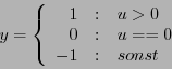
Eine symmetrische lineare Schwellwertfunktion (mit Sättigung) bekommt man mit (vgl. Bild 3.9) der Formel:

$\begin{displaymath} y = \left \{ \begin{array}{r@{\quad:\quad}l} 1 & u > 0\\ 0 & u == 0\\ -1 & sonst \end{array}\right. \end{displaymath}$

**Figure 3.10:** Aktivierungs als schrittweise Funktion mit Schranken (Sättigung)
$\includegraphics[width=3.0in]{actPiece.eps}$

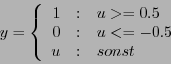
Eine schrittweise lineare Schwellwertfunktion (mit Sättigung) bekommt man mit (vgl. Bild 3.10) der Formel:

$\begin{displaymath} y = \left \{ \begin{array}{r@{\quad:\quad}l} 1 & u >= 0.5\\ 0 & u <= -0.5\\ u & sonst \end{array}\right. \end{displaymath}$

**Figure 3.11:** Aktivierungs als Sinusfunktion
$\includegraphics[width=4.0in]{actSin.eps}$

Eine sinusförmige Aktivierungsfunktion (mit Sättigung) bekommt man mit (vgl. Bild 3.11) der Formel:

$\begin{displaymath} y = \sin(u) \end{displaymath}$

**Figure 3.12:** Aktivierungs als logistische Funktion (sigmoidal) mit slope s= 0.5/ 0.75/ 0.9
$\includegraphics[width=4.0in]{actLog.eps}$

Eine alternative Form einer sinusförmigen Aktivierungsfunktion (mit Sättigung) bekommt man mit (vgl. Bild 3.12) der Formel (

als Anstiegswinkel ('slope')):

$\begin{displaymath} y = \frac{1}{1 + exp(-su)} \end{displaymath}$

**Figure 3.13:** Aktivierungs als probabilistische Funktion mit Pseudotemperatur T= 0.25/ 0.5/ 0.75
$\includegraphics[width=4.0in]{actProb.eps}$

Eine probalilisische Aktivierungsfunktion bekommt man mit (vgl. Bild 3.13) der Formel (

als Pseudotemperatur):

$\begin{displaymath} y = \frac{1}{1 + exp(-u/T)} \end{displaymath}$

**Figure 3.14:** Aktivierungs als tangens hyperbolicus
$\includegraphics[width=4.0in]{actTanhGrid.eps}$

Eine Aktivierungsfunktion mit dem tangens hyperbolicus

bekommt man mit (vgl. Bild 3.14) der Formel (

als Pseudotemperatur):

$\begin{displaymath} y = \tanh(u) \end{displaymath}$