Attention : The text is not a complete representation of the oral lecture !!!
                        The text ist  finished, but there can be improvements of the definitions
                        in the future.
                        

1. Introduction

In the preceding lecture we have selected adaptive binary tree-structures as the most interesting candidates for possible answeres to a lot of interesting real-world problems. This involves some basic theoretical concepts which we have to introduce here as necessary framework for the upcoming concrete structures.

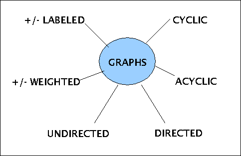
From a practical point of view there are onyl a few basic properties of graphs which are important:

In an informal way one can describe these properties as follows:

1. Graphs := a set of vertices (nodes) which are connected by edges (arcs) with no special direction; not all vertices must be connected. Following the edges you are generating a path, which can lead back to a vertex which you have already passed.




2. Undirected/ directed := a graph becomes a directed graph, if you can follow the edges only in one direction




3. Cyclic/ acyclic := if you are following the edges of a graph and you will never return to a vertex you have already passed, then the graph is acyclic.




4. Not labeled/ labeled := a label is some information attached to a vertex (node). Example: you have a sheet of paper with vertices and edges drawn on it and the vertices e.g. have attached names of cities.




5. Not weighted/ weighted := a weight is some additional information attached to an edge. This is usual an information about the costs to pass this edge from one vertex to the other (e.g. 'the time to travel', the 'expense to reach', 'the work to do', 'the amount of energy to spent' etc.).

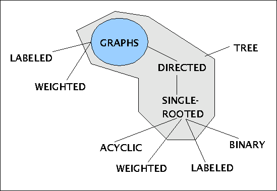
As you can easily see are these basic properties independent one from another; a graph can be undirected and acycliy, with or without labels or weights. Thus you can mix up these basic properties as you need them. Some of the more often occuring combinations are given in the following diagram:

As you can see from this diagram are trees a special case of graphs; trees are that subset of graphs which are directed and have only one root. The root is the only node from which you can reach all other nodes. Trees can then have additional properties like to be acyclic, labeled, weithted or to be binary. Binary means that from each node in a binary tree you have at most two possible continuations. Again it holds that all these properties are independed insofar you can mix these properties as needed.

Because of this independent character of most of these properties --to be 'single rooted' depends from beeing directed-- it is difficult to give a complete systematic of formal concepts; thus we will introduce these concepts as possible 'building blocks' of larger structures.

2. Formal Definitions

First we will give some formale definitions of the mostly used concepts. As usual, there are several possibilities how to define a concept. We have tried to cover the common usage in the textbooks; but there are concepts which rarely are explicitly defined, thus we have given one possible formula. It is up to you to improve these concepts if this would be necessary for some special applications.

2.1 (Unlabeled/ Unweighted) Graphs

The basic concept is the concept of graphs.

1. (UNLABELED/ UNWEIGHTED) GRAPH(g) iff g = <V,E>

   with

   • V := finite set of vertices (nodes)

   • E := finite set of edges (arcs)

   • E C V x V

   • In the general case it holds: REFLEXIVE(E): (x,x) in E &
     SYMMETRICAL(E): (x,y) in E ==> (y,x) in E

   
   

2. Def: GRAPH(g) ==>
   vertices(g) = g₁




3. Def: GRAPH(g)==>
   edges(g) = g₂




4. Def: ADJACENT(x,y,k,g) iff GRAPH(g) & k in edges(g) & k = (x,y)




5. Def: CONNECT(k, x,y,g) iff ADJACENT(x,y,k,g)




6. Def: ENDPOINTS(x,y,k,g) iff ADJACENT(x,y,k,g)




7. Def: INCIDENT(x,y,k,g) iff ADJACENT(x,y,k,g)




8. Def: NEIGHBOURS(x,y) iff (E:k,g) ADJACENT(x,y,k,g)




9. Def: SIMPLEX(g) iff GRAPH(g) & (A:x,y)( x,y in vertices(g) ==> NEIGHBOURS(x,y))




10. Def: DIRECTED_GRAPH(g) --DG(g)-- /* also called Digraph */ iff GRAPH(g) & ~SYMMETRICAL(edges(g)).




11. Def: HEAD_OF(x,k,g) iff ( DG(g) & k in edges(g) & x = pr1(k) )




12. Def: TAIL_OF(y,k,g) iff ( DG(g) & k in edges(g) & y = pr2(k) )




13. Def: LEADS_FROM_TO(x,y,k,g) iff HEAD_OF(x,k,g) & TAIL_OF(y,k,g)




14. Def: PREDECESSOR_OF(y,x,g) iff (E:k)( LEADS_FROM_TO(y,x,k,g) )




15. Def: SUCCCESSOR_OF(y,x,g) iff (E:k)( LEADS_FROM_TO(x,y,k,g) )




16. Def: indegree(x,g) = |{y| PREDECESSOR_OF(y,x,g) }|




17. Def: PATH(p,g) iff DG(g) & SEQUENCE(p) & rng(p) C vertices(g) & (A:i,j)( i,j in dom(p) & j=i+1 ==> (p_i,p_j) in edges(g))




18. Def: PATH(p,g) ==>
    length(p) = |dom(p)|-1 /* Number of edges, not vertices! */




19. Def: HEAD_OF_PATH(x,p,g) iff PATH(p,g) & x = p₁




20. Def: END_OF_PATH(y,p,g) iff PATH(p,g) & x = p_length(p)+1




21. Def: CYCLIC_PATH(p,g) iff PATH(p,g) & (E:x,y)( HEAD_OF_PATH(x,p,g) & END_OF_PATH(y,p,g) & x=y )




22. Def: GRAPH(g) ==>
    successors(x,g) = {y| (E:p)( PATH(p,g) & HEAD_OF_PATH(x,p,g) & END_OF_PATH(y,p,g) )}




23. Def: SUBGRAPH(g',g) iff GRAPH(g) & (E:x,n,a)( g' = <n,a > & x in vertices(g) & n = {y| successors(x,g)} & a = n x n cut edges(g))

2.2 Directed Acyclic Graphs

24. Def: DIRECTED_ACYCLIC_GRAPH(g) --DAG(g)-- iff DG(g) & ~(E:p)( CYCLIC_PATH(p,g))

2.3 Labeled/ Weighted Graphs

The concept of graphs which is used in practice is usually more complex than shown before. This is caused by the fact that in many applications one is not only interested in the 'graph structure as such' (vertices connected by edges), but one has to connect the vertices and the edges with additional information. These additional information can be 'costs' (or 'weights') of passing from one vertex to another or can be information hosted by a vertex at a certain position represented as a vector of values, also called 'label'. Examples are the names of cities which are the labels of vertices in a graph or the key-value-pairs of binary search-trees.

To meet these requirements one has to enlarge the formal concept of graphs by additional labels and costs.

25. LABELED/ WEIGHTED GRAPH(g) --LGRAPH(g) or LG(g)-- iff g = << V, R, VL, d1, EL, d2 >,E>




with

• V := finite set of vertices (nodes)

• R := finite set of root vertices

• VL := finite set of vertex labels

• d1 := dimensionality of vertex labels

• EL := finite set of edge-labels ('costs', 'weights')

• d2 := dimensionality of edge labels

• E := finite set of edges (arcs)

• R C V

• E C ((V x VL^d1) x (V x VL^d1)) x EL^d2
  
  Thus an element of the set E has the general form: ((x,<vl₁, ... ,vl_d1>),(y,<vl₁, ... ,vl_d1>)),<el₁, ... ,el_d2>)
  this represents an edge with vertices x and y and vertex x has the label <vl₁, ... ,vl_d1> and vertex y has the label <vl₁, ... ,vl_d1> and the cost of passing from x to y (or back) is given by <el₁, ... ,el_d2>




26. Def: LGRAPH(g) ==>
    vertices(g) = g_1.1




27. Def: LGRAPH(g) ==>
    roots(g) = g_1.2




28. Def: LGRAPH(g) ==>
    vertex-labels(g) = g_1.3
    

29. Def: LGRAPH(g) ==>
    vertex_label_dimensionality(g) = g_1.4
    values(g) = vertex-labels(g)




30. Def: LGRAPH(g) ==>
    edge-labels(g) = g_1.5
    costs(g) = weights(g) = edge-labels(g)




31. Def: LGRAPH(g) ==>
    edge_label_dimensionality(g) = g_1.6
    

32. Def: LGRAPH(g)==>
    edges(g) = g₂




33. Def: LGRAPH(g)==>
    LABELED_EDGE(le,g) iff le in edges(g)




34. Def: LGRAPH(g)==>
    LABELED_VERTEX(lv,le) iff LABELED_EDGE(le,g) & lv = proj1(proj1(le)) or lv = proj2(proj1(le))




35. Def: LGRAPH(g)==>
    WEIGHTS(w,le) iff LABELED_EDGE(le,g) & w = proj2(le)
    COSTS(c,le) iff WEIGHTS(w,le)




36. Def: LGRAPH(g) & LABELED_EDGE(le,g) ==>
    head(le) = proj1(proj1(le))
    tail(le) = proj2(proj1(le))




37. Def: LGRAPH(g)==>
    NREFLEXIVE(E) iff E = edges(g) & (A:e)(LABELED_EDGE(e,g) ==> head(e) = tail(e) )




38. Def: LGRAPH(g)==>
    NSYMMETRICAL(E) iff E = edges(g) & (A:e)(LABELED_EDGE(e,g) ==> (E:e')(head(e) = tail(e') & tail(e) = head(e')) )




39. Axiom: LGRAPH(g)==> NREFLEXIVE(edges(g)) & NSYMMETRICAL(edges(g))




40. Axiom: LGRAPH(g)==> & r in roots(g) ==> ~(E:e)( e in edges(g) & r = tail(e) )




41. Def: LGRAPH(g)==>
    ADJACENT(x,y,k) iff k in edges(g) & x= pro1(pro1(k)) & y = pro2(pro1(k))




42. Def: Def: LGRAPH(g)==>
    CONNECT(k, x,y) iff ADJACENT(x,y,k)
    ENDPOINTS(x,y,k) iff ADJACENT(x,y,k)
    INCIDENT(x,y,k) iff ADJACENT(x,y,k)




43. Def: LGRAPH(g)==>
    NEIGHBOURS(x,y) iff (E:k) ADJACENT(x,y,k)




44. Def: LSIMPLEX(g) iff LGRAPH(g) & (A:x,y)( x,y in vertices(g) ==> NEIGHBOURS(x,y))




45. Def: LABELED_DIRECTED_GRAPH(g) --LDG(g)-- iff LGRAPH(g) & ~NSYMMETRICAL(edges(g)).




46. HEAD_OF(x,k,g) iff ( LDG(g) & k in edges(g) & x = head(k) )




47. TAIL_OF(y,k,g) iff ( LDG(g) & k in edges(g) & y = tail(k) )




48. LEADS_FROM_TO(x,y,k,g) iff ( HEAD_OF(x,k,g) & TAIL_OF(y,k,g) )




49. PREDECESSOR_OF(y,x,g) iff (E:k)( LEADS_FROM_TO(y,x,k,g) )




50. Def: SUCCCESSOR_OF(y,x,g) iff (E:k)( LEADS_FROM_TO(x,y,k,g) )




51. Def: LPATH(p,g) iff LDG(g) & SEQUENCE(p) & rng(p) C vertices(g) x vertex_labels(g)^k & (A:i,j)( i,j in dom(p) & j=i+1 ==> (E:w)( w in weights(g)^s & ((p_i,p_j),w) in edges(g))




52. Def: LPATH(p,g) ==>
    length(p) = |dom(p)|-1 /* Number of edges, not vertices! */
    

53. Def: values(p,g) = { (i,v) | i in dm(p) & p_i in p & ((p_i, p_j),v) in edges(g) }


wlength(p) = SUM(i=1,length(p)) v_i in values(p,g) /* summing up all costs on the path */



54. Def: HEAD_OF_LPATH(x,p,g) iff LPATH(p,g) & x = p₁




55. Def: END_OF_LPATH(y,p,g) iff LPATH(p,g) & y = p_length(p)+1




56. Def: LABELED_CYCLIC_PATH(p,g) iff LPATH(p,g) & (E:x,y)( HEAD_OF_LPATH(x,p,g) & END_OF_LPATH(y,p,g) & x=y )




57. Def: LABELED_DIRECTED_ACYCLIC_GRAPH(g) --LDAG(g)-- iff LDG(g) & ~(E:p)( LABELED_CYCLIC_PATH(p,g))

2.4 Labeled Trees

Simply speaking is a labeled tree in the general case a labeled directed acyclic graph with only one root-vertex from which all vertices of the tree can be reached.

58. LABELED_TREE(t) --LT(t)-- iff LDAG(t) & |roots(t)| = 1 & LSIMLPLEX(t)

There is some special terminology connected with trees different to graphs:

59. Def: LABELED_TREE(t) ==>
    nodes(t) = vertices(t)




60. Def: PARENT(x,y) iff PREDECESSOR_OF(x,y)




61. Def: CHILD(y,x) iff SUCCCESSOR_OF(y,x)




62. Def: children(x) = {y| CHILD(y,x) }.




63. Def: LEAF(l,t) iff ( LABELED_TREE(t) & l in nodes(t) & ~(E:e)( e in edges(t) & l = head(e) ) )




64. Def: LABELED_TREE(t) ==>
    leafs(t) = {x| LEAF(x,t) }




65. Def: LABELED_TREE(t) ==>
    inner_nodes(t) = nodes(t)\leaves(t)




66. Def: LABELED_TREE(t) ==>
    PATH_TO(p,x) iff LPATH(p,t) & (E:r)( r in roots(t) & HEAD_OF_LPATH(r,p,t) & END_OF_LPATH(x,p,t) )




67. Def: LABELED_TREE(t) ==>
    PATH_FROM(p,x) iff LPATH(p,t) & (E:l)( LEAF(l,t) & HEAD_OF_LPATH(x,p,t) & END_OF_LPATH(l,p,t) & ~(E:l',p')( LEAF(l',t) & LPATH(p',t) & HEAD_OF_LPATH(x,p',t) & END_OF_LPATH(l',p',t) & lenth(p) < length(p') ))




68. Def: LABELED_TREE(t) & PATH_TO(p,x) ==>
    depth(x) = length(p)




69. Def: LABELED_TREE(t) & PATH_FROM(p,x) ==>
    height(x) = length(p)




70. Def: LABELED_TREE(t) ==>
    ORDER(n,t) iff (A:x)( x in nodes(t) ==> |children(x)| < n )




71. Def: LABELED_TREE(t) & PATH_FROM(p,x) ==>
    height(t) = length(p) iff x in roots(t) & ~(E:p')( PATH_FROM(p',x ) & length(p') > length(p) )




72. Def: COMPLETE(t) iff LABELED_TREE(t) & (E:n)( ORDER(n,t) &

    
    

    • (A:x,p)( PATH_TO(p,x) & LEAVE(x,t) ==> depth(x) = n ) &

    
    

    • (A:i,p)( PATH_TO(p,x) ) & ~LEAVE(x,t) & i in n & depth(x)= i ==> |children(x)| = n )

    
    
    )

2.5 Trees

Trees are simplified forms of labeled trees:.

73. TREE(t) iff LT(t) & vertex_labels_dimensionality(t) = 0 & edge_labels_dimensionality(t) = 0

2.6 Labeled Binary Trees

A binary tree can simply de defined as:

74. LABELED_BINARY_TREE(t) --LBT(t)-- iff LABELED_TREE(t) & ORDER(2,t)

2.7 Binary Trees

75. BINARY_TREE(t) --BT(t)-- iff TREE(t) & ORDER(2,t)

2.8 Binary Search Trees

A binary search tree is informally something 'between' a labeled binary tree and a binary tree. A binary search tree has no weights, but 2-dimensional labels with the first elemet of the label called 'key' and the second element of the label called 'value'. These labels are distributed over the tree in a way that they follow some order.

76. Def: BINARY_SEARCH_TREE(t) --BST(t)-- iff LABELED_BINARY_TREE(t) & vertex_labels_dimensionality(t) = 2 & edge_labels_dimensionality(t) = 0
    




77. Def: BINARY_SEARCH_TREE(t) & LABELED_EDGE(e,g) & LABELED_VERTEX(v,e) ==>
    label(v) = proj2(v)
    key(v) = proj1(label(v))
    value(v) = proj2(label(v))
    




78. Def: BINARY_SEARCH_TREE(t) & x in nodes(t) x vertex_labels(t)^{vertex_labels_dimensionylity(t)} ==>
    keys(x,t) = {k| (E:y)( y in successors(x,t) & k=key(y) ) }
    




79. Axiom: BINARY_SEARCH_TREE(t) & a in nodes(t) & x,y in children(a) ==> (A:i)( i in keys(x,t) ==> ~(E:j)( j in keys(y,t) & j > i )) )
    /* In this definition no 'left-right-order' has bee used */

2.9 Balanced Binary Search Trees

Will be explained in the next lectures when we will deal with AVL-trees and Red-Black-trees.

3. Typical Problems with Graphs

Many problems can succesfully be represented within the framework of graphs. In the following we are giving a short overview of some of these problems which are of practical importance. Some of these problems we will analyze further in the upcoming lectures, but not all, because the time is too short.

3.1 Topological Sorting

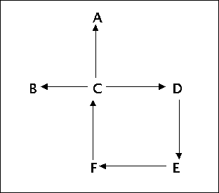
A digraph can be interpreted as a weakly ordered structure where the direction of the edge is representing the 'order'. In a topological sort one maps the set of vertices with cardinality |V| in a subset of the natural numbers with top_sort: V ---> |V| such, that the ordering holds in |V|. It follows from this, that a topological sorted graph can not have cycles, because in this case one would have a pair like (C,C) which is contradicting the ordering relation (see diagram).

More detailed:

Assume that an edge is a weakly ordered structure like '<'. It holds e.g. that TRANS(<) & ¬SYM(<). Thus if we translate the graph from the diagram into relational expressions we are getting the following subset: C < D, D < E, E < F and F <C. From C < D, D < E, E < F it follows by TANSITIVITY that C < F. But then we have a contradiction because C < F and F <C causes the statements SYM(<) and ¬SYM(<).

Thus it follows that a topological sorted graph is acyclic and therefore includes only one vertex x with indegree(x) = 0.

Therefore one can use an algorithm for testing of topological sorting to check the property of being cyclic or acyclic.

3.2 Transitive Closure

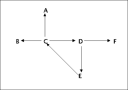
The transitive closure of a graph is connected to the problem of finding all connections between vertices of a graph. A possible definition that c is the reflexive transitive closure of g could be: RTC(c,g) iff GRAPH(g) with g = <V,E > & c = <V,E* > such that (v,v') in E* iff there is a path in g from v to v'.

In the diagram below there are the following elements in E*: {(C,D,), (C,F),(C,E),(C,C),(C,A),(C,B), (D,F), (D,E), (E,C)}

Thus to compute the transitive closure of a graph g can be a starting point to find some optimizations.

3.3 Traversing a Graph

Traversing a graph g means generally to 'visit' every vertex from some arbitrarily selected starting point x at least once. A simple, linear version of such a search could be to take the set E of edges(g), organize the set as a list and look to every edge of E. If we declare the edges(g) in the beginning as the border-set distinguished from the visited-set, then the search continus until the border-set is empty.

One interesting aspect can be to search in a graph g all connected subgraphs. One can elaborate these searches to reveal more about the struture of the graph being searched.

3.4 Shortest Path/ Critical Path

In many cases is the edge (v,v') of a graph g connected with some properties which represent the 'length' or the 'costs' or something else of moving from vertex v to vertex v'. In these cases it is interesting to know the 'shortest' path in the sense to have the path with the minimal 'length' or minimal 'costs'.

A special case is the 'critical path'. In most projects depends the final vertex --the goal-- mostly not only from one single path but from the interactions of different paths where one path is depending from some other paths. Here it is an interesting question what is the shortest path constrained by all the other paths.

3.5 Minimal spanning Trees

Related to the question of shortest path in a graph g is the question of a minimum spanning tree. A spanning tree of an undirected graph g is a tree t formed by graph edges that connect all the vertices of graph g. The cost of the spanning tree ist the sum of the costs of the edges in the tree. The minimum spanning tree is a connected subgraph of g that spans all vertices at minimum cost. A graph g is connected if there exists a path p for all vertices in g. Because a minimum spanning tree of a subgraph of g exists only if the the subgraph of g is connected one can use the algorithm for the computation of mimum spanning trees as a test of connectivity.

3.6 Capacities in Networks

Another interesting problem is the question of the computation of the flow of certain capacities (cars, passenger, data-pakets, goods, visitors...) through a network.

3.7 Inheritance-Graphs

A heritage-graph represents the relationship between parents and children over generations, where the vertices are labeled (names, dates, living/ dead,...) and with regard to these information one has to compute special predicates representing special types of relationships and the amount of inhertance someone can inherit by law.

3.8 Mapping of Graphs

A very common problem is the optimal mapping of employees with certain skills to tasks in projects, or of teaching people to lectures, resources and time-slots.

4. Exercices

In the following you will find a list of topics taken from the preceding text. Try to worke out the following tasks with regard to some of the mentioned topics:

1. Create an example-grah which could be an example for the selected topic..




2. Try to give a formal definition of this graph.




3. Try to find an algorithm to solve the problem.




4. Describe whiche data structure you are using to represent the graph and which data structures to support the actual search-operations of the algorithm.




5. Compute the complexity of your algorithm.




6. In which way can you minimize the complexity of your algorithm with regard to your datastructures?

List of possible topics:

1. Topological Sorting




2. Transitive Closure




3. Traversing a Graph




4. Shortest Path




5. Critical Path




6. Minimal spanning Trees




7. Capacities in Networks




8. Inheritance-Graphs




9. Mapping